User Area > Advice
Finite Element Equilibrium
In
terms of finite element equilibrium, there are two important
properties that are always satisfied by the finite element
solution using either a coarse or a fine mesh. To describe
these properties consider the following portion of a mesh
under the application of an arbitrary force, the four elements
(1,2,3,4) share the same node (i).
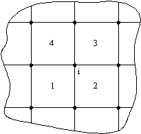
The
following diagram, representing an exploded view of these
four elements, shows the forces obtained at the nodal position
(i) and those on element (2).
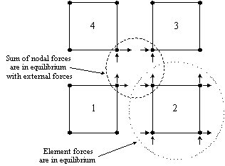
The
two properties may now be defined as
�
Nodal
point equilibrium: At any node, the sum of the internal
element point forces is in equilibrium with any external
loads that are applied to the node. The internal forces
include the effects due to body forces, surface tractions,
initial stresses, concentrated loads, inertia and damping
forces, and reactions. Thus, for an externally non-loaded
node in a linear static analysis, such a summation will
be zero.
�
Element
equilibrium: Each element is in equilibrium under its internal
forces
Nonlinear analyses may produce out-of-balance residual forces at a node,
depending on the degree of convergence obtained during the solution.
For a well-converged solution, however, these are insignificant.
See nonlinear
iterative strategy for more information.
Although
nodal and element equilibrium is achieved as described above,
in a general finite element analysis, differential equilibrium
(e.g. stress equilibrium) is not necessarily achieved at
all points of the continuum considered – most notably
at the shared boundaries of elements. The reason is as follows…
In
the displacement-based finite element method, a C0
continuous approximation for the displacements is assumed
within each element. This means that the displacements at
any point in a mesh will be continuous and ensures that
no gaps appear between elements. The element stresses are
calculated using derivatives of the displacement which means
that they will not necessarily be continuous and give rise
to inter-element discontinuities or “jumps” in
stress between adjacent elements (an example is given in
“Implication:
For
the same reasons that element stresses are not continuous
across element boundaries, the element stresses at the surface
of a finite element model are, in general, not in equilibrium
with the external applied tractions. Again, this effect
is minimised with mesh refinement.
Experience
has shown that the most accurate locations for stress output
are the Gauss points. Nodal points, which are the most accessible,
are actually the worst output location for stresses. Reasons
have been given above, but include the fact that shape functions
tend to behave badly at element extremities and it is reasonable
to expect that the shape function derivatives (i.e. strains/stresses)
sampled in the interior of the element would be more accurate
than those sampled at the periphery of the element.
This
evokes the question of how to obtain accurate stress results
from a finite element model?
Implication:
Smoothed or Unsmoothed Stress Contours?
One
method for obtaining reasonable nodal stress output is by
extrapolating the “exact” stresses at Gauss points
to the nodal positions using the element shape
functions. Consider the following diagram, representing
the same exploded view of the four elements shown earlier.
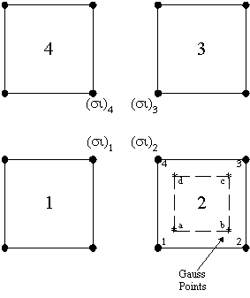
For
element 2, the nodal stresses at nodes (1,2,3,4) are obtained
by
- Defining
a fictitious element (shown by the dashed lines) with
nodes at the element Gauss points (a,b,c,d)
- Extrapolating
the Gauss point stresses to the nodal points of the real
element (1,2,3,4) using the displacement shape
functions of the fictitious element, i.e.

Where N is the
number of Gauss points, and subscripts i and I denote nodal
and Gauss point values respectively.
The accuracy of the extrapolation procedure is dependent on both the presence
of a reasonably uniform stress field and the type of shape
function used in the element chosen. For instance, a
high stress gradient across an element would be more likely
to extrapolate incorrectly, particularly if a linear shape
function element is being used.
This
procedure is carried out for the other elements and the
nodal stresses at the common node (i) are obtained as (si)1,
(si)2,
etc. As pointed out above, these stresses are not usually
equal and a single “averaged” or “smoothed”
nodal stress value is obtained using

When
this procedure is carried out for all nodes in an element
assembly, the ensuing averaged stress values provide a reasonable
approximation to a continuous stress field. This is a straightforward
and economic solution and works well on the whole. See later
for more details on the circumstances that smoothing should
not be used. This is the default method used in MODELLER
when smoothed results are selected in the contour layer
properties. If smoothed results are not selected then the
extrapolation procedure is still performed, but the averaging
process is omitted. The averaging procedure is also
carried out when the "values" and
"loading" layers are selected.
Note
that, for shell elements, the local Gauss point stresses
and strains are transformed to global stresses and strains
before extrapolation to the nodes. The mean global stresses
are then transformed to the local shell system at the nodal
point before evaluation of the nodal stress resultants.
Other
methods are available, based on a least squares fit over
the integration point stress values of the elements. The
least squares procedure might be applied over the patches
of adjacent elements or even globally over a whole mesh.
However, if the domain over which the least squares fit
is applied involves many stress points, the solution will
be expensive and, in addition, a large error in one part
of the domain may affect rather strongly the least squares
prediction in the other parts.
In
general, it is recommended to display unsmoothed stress
contours at an early point during the processing of results.
In this way, severe stress discontinuities between elements
will be apparent and the possible requirement of mesh refinement
and/or the use of higher order elements may be considered.
In
areas of interest where the stress results will be used
in the design process, smoothed contours would ideally be
similar to unsmoothed contours. The inference from this
being that a smooth stress transition across the element
boundaries indicates that the stress distribution in the
structure is being simulated sufficiently accurately. For
sections of the model that are not of interest, a coarser
mesh would normally be used and such a comparison in these
areas would typically give significantly different contours
- smoothed contours appearing more like a patchwork quilt!
The
nodal averaging technique is sufficiently robust that such
stress values will tend to be pretty much those that would
be obtained at the same location with mesh refinement –
as long as the element mesh is reasonably uniform.
At
all times, it is imperative to remember that the finite
element method is an approximate numerical technique (albeit
a good one!) and that smoothed stress results can give good
results but need careful attention.
Implication:
Limitations of the averaging scheme
In
addition to taking no account of the size of the adjacent
elements, the averaging method must not be used
-
At
mesh locations in which geometric or material properties
change.
-
For
local or global stress output for shell elements that are
non-planar. At the intersection of the three elements
shown below, for instance, it is invalid to add the
local sy stresses.
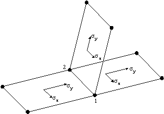
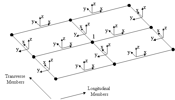
Consider the situation
in which Mx results have been selected for display
using the “values” layer in MODELLER and both
transverse and longitudinal members are active. The averaged
value displayed at the central node number (1) will be comprised
of the local Mx values from the two longitudinal
and two transverse members that connect to this node. It
must be noted that the Mx values are local to
the elements (as shown in the diagram), so that the Mx
values for the longitudinal members act at 90 degrees to
the Mx results in the transverse members. This
means that the averaged values will be meaningless since
the Mx results from the longitudinal members
will be averaged with the Mx values of the transverse
members that are acting in a completely different direction.
One remedy would be to ensure that the Mx values
from the longitudinal members were combined with the more
appropriate My values from the transverse members
– results that are acting in the same direction. This
remedy is not actually workable, and so the use of the “diagrams”
layer or the proper use of “advanced selection”
should be invoked if the “values” or “contour”
layers are actually required.
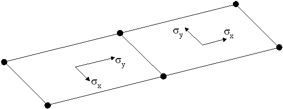
In this case, averaging the sx stress
components at one of the two adjoining nodes will result
in a sx stress being averaged with a sy stress - the resulting
smoothed stress being clearly incorrect. This may be overcome
for most quadrilateral meshes by modifying the element
axes (cycling or reversing the underlying feature axes).
For triangular elements, however, no amount of cycling
will obtain a consistent set of local element axes - as
will be observed in the following figure.
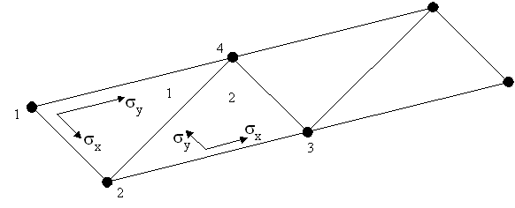
In the case of triangular
elements, the stress results should be transformed appropriately.
Element results that are displayed in a global axis system
will not be affected by such local element axis problems.
-
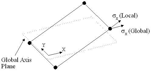
Where a shell surface is curved or does
not lie in one of the global axis planes (even if flat),
stresses will be difficult to interpret in Modeller since
the chosen stress component may "intersect" the element
plane at an awkward angle. In such cases the stresses
should be transformed to an orientation corresponding
to the shell plane or a direction-independent stress measures
such as principal or von Mises. The problem can be seen
in the following diagram in which the default sx (global)
direction can be seen to be at an orientation that is
unlikely to be in a helpful orientation when compared
to the more usual orientation of the local sx direction.
Implication:
Removal of elements affects the stress contours
-
An
implication of the averaging process is that when contouring
selected parts of the structure, the elements that have
been removed from the active list will no longer make a
contribution to the averaging process. Depending on the
relative size of the stress contributions that are now missing,
the contours at the selected element boundary may change
significantly. Unsmoothed results do not behave in this
manner.
Additional
Links
Finite
Element Theory Contents
|