User Area > Advice
Shape Function Interpolation
Displacement shape or interpolation
functions are a central feature of the displacement-based
finite element method. They primarily characterise the assumptions
regarding the variation of displacements within each element.
Because of their relationship with displacements, the variation
of both strains and stresses is also consequently defined.
The basic assumption of the finite element
method is that the subdivision of a complex physical structure
into the assembly of a number of simple “elements”
will approximate the behaviour of the structure. Because
of this subdivision, each finite element need not attempt
to simulate the complex behaviour of the whole structure
but, rather, assumes a relatively simple displacement variation
so that the sum of the individual finite element responses
approximates the response of the whole structure.
Shape functions are polynomial expressions.
Any order of polynomial can theoretically be used but, in
general, linear and quadratic variations are most common.
It is from the order of the shape function polynomial that
the terms linear and quadratic elements originate.
A consequence of these assumed displacement
variations enables the finite element method to be able
to solve the equilibrium equations at discrete points, thus
transforming a continuous “physical” system (having
infinite degree of freedom) into something manageable for
numerical procedures.
Typically, LUSAS uses Lagrangian shape functions
which provide C(0) continuity between elements (primary variables
only, and not their derivatives, are continuous across element
boundaries). Shape functions are defined in terms of the natural
coordinate system (x) for line
elements (bars, beams), (x, h) for
surface elements (shells, plates, plane membranes) (x,
h, z) and for volume elements (solids).
For many two-noded line elements a linear
variation is assumed as follows


Where N1 and N2
are the shape functions at nodes 1 and 2 of the element
respectively (the order being dependent on the element node
numbering). Diagrammatically, their variation is as follows
Linear variations are also used on four-noded
surface elements as follows
Three-noded line elements typically
assume a quadratic variation as follows


Where N1, N2 and N3
are the shape functions at nodes 1, 2 and 3 of the element
respectively. Diagrammatically, their variation is as follows
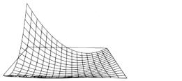
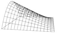
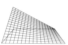
Quadratic variations are also used on
eight-noded
surface elements. The following diagrams show the variations
of the shape functions at both corner and midside nodes
Shape functions need to have the following
characteristics
This means that the value of each shape
function evaluated at its nodal position must be unity.
For example
Requires that the values of each shape function,
evaluated at the other nodes must be zero. That is


The sum of all the shape functions, evaluated
at any point must be unity. That is
Furthermore, to ensure that a finite element
convergences to the correct result, certain requirements
need to be satisfied by the shape functions, as follows
The displacement function should be such
that it does not permit straining of an element to occur
when the nodal displacements are caused by rigid body displacement.
This is self evident, since an unsupported structure in
space will be subject to no restraining forces
The displacement function should be of such
a form that if nodal displacements produce a constant strain
condition, such constant strain will be obtained. This is
essential since a significant mesh refinement will cause
near-constant strain conditions to occur in elements and
they must be able to handle this condition correctly
The displacement function should ensure
that the strains at the interface between elements are finite
(even though indeterminate). By this, the element boundaries
will have no “gaps” appear between them and, hence,
will show a continuous mesh.
The following sections deal with some of
the more frequently encountered practical implications that
are related to the use of shape functions.
Implication: The evaluation of element displacements
The isoparametric
element formulation assumes that

Where {u} are the displacements at any point
within an element and {d} are the displacements at the nodes
of an element.
This equation relates the displacements
at any point within an element to the nodal displacements
according to the element shape function [N]. Therefore,
the displacement at any point (x) in
a 2-noded line element can be obtained from the nodal values
using the following equation
If this element is fully fixed at one end
(d1=0) and sustains a displacement of 2 at the
other end (d2=2), the displacement at the centre
of this element (x=0) would be
given thus
i.e. half the end displacement as expected.
The same can be done with any quantity that
varies across an element, for example, coordinates, strain,
stress, and thickness.
Consider a 3-noded element that uses a quadratic
shape function variation of the form
The quadratic terms (x) in thus giving a corresponding quadratic variation
of displacement over the element. The strain variation can
be defined as

Where [B] is that strain-displacement matrix
and {d} are the three element axial displacements. It can
be seen from the x terms that
the strain is now a linear variation – as will be the
stress variation. In a similar manner, for a linear element,
the strain and stress variation will be constant.
This has a direct bearing on the type of element
to be chosen for an analysis. For instance, consider a bar
element under the action of a constant uniformly distributed
load along the length of the element. The resulting axial
force variation will be theoretically linear as in the topmost
picture of the following diagram.
If this bar is modelled using linear elements
(i.e. linear terms in the shape function), the axial force
will be approximated by a constant, “stepped”
response in each element, since the shape function derivatives
only contain constant terms. A quadratic element (i.e. quadratic
terms in the shape function) will, however, support a linear
response and provide the correct answer directly, since
the shape function derivatives contain linear terms. Thus,
the exact solution can be obtained with a relatively small
number of elements (or even with one element only) if the
actual strain field can be matched by the shape functions
of the element that is being used. In the above example,
the shape function derivative terms did indeed match the
linear strain of the actual analysis.
A frequent observation when inspecting force
output at a simply supported section of a structure is to
find (unexpectedly) non-zero values. Depending on the degree
of mesh refinement, these values can be significant compared
to the peak values. The reason is directly related to the
above discussion. For example, if the force distribution
is at least quadratic in form and linear elements are used
(typically supporting a constant force distribution), a
stepped response will be seen – hence the non-zero
values – these constant values represent an average
of the force distribution and, if summed across the structure
would be found to be equilibrium. The use of quadratic elements
will improve the situation, but even these will not be able
to match 3rd order or higher force distributions
without a measure of mesh refinement performed.
In spite of this sort of discrepancy, it should
be noted that, during the solution stage, the equilibrium
equation is used ({f}= [K] {d}) to ensure that the product
of the stiffness matrix and the computed displacements exactly
balances the externally applied forces. This means that, unless
there are pertinent warnings or errors output during the solution,
static equilibrium will have been fully achieved. Moreover,
the derived quantities of strain and stress will also be found
to be in equilibrium – but not necessarily according
to an expected distribution as noted in preceding paragraphs.
See “Finite
Element Equilibrium” for more information.
Similar difficulties can be observed when
attempting to compare the reactions at a location in a structure
with the element force output at the same location. The
explanation in most cases is, again, related to the order
of shape function that has been used to formulate the element.
See “finite element equilibrium” for more information.
The remedies are to either increase the
number of linear elements used (and reduce the size of the
“step change” between each element) or change
to quadratic elements (to more closely match the actual
variation). The specific element NOTES section in the LUSAS
Element Library Manual will typically give details on the
variation of force that is supported by each element.
Apart from the consideration of element
selection related to the order of shape function, quadratic
elements would be recommended in the presence of high degrees
of plastic strain since they are less susceptible to “locking”.
Linear elements, however, would be recommended when the
stress distributions anticipated are constant or linear.
Such elements are computationally cheaper and, in such circumstances,
render the use of higher order elements unnecessary.
For a discussion on the effects of stress
smoothing (averaging) in the presence of discontinuous stress
fields between elements see “finite
element equilibrium”.
Implication: Nodal Temperature Loading With Temperature
Dependent Materials
Although the temperature loading is defined
at element nodes, it is actually used by LUSAS at a Gauss
point level. The nodal temperature loading is interpolated
from the nodes to the Gauss points using the element shape
functions.
The presence of significant temperature
loading distributions over higher order elements can cause
negative temperature loading to be applied at the Gauss
points – even though the applied temperature field
is entirely positive in magnitude. Such negative temperatures
can be unexpectedly out of the user-specified temperature
dependent material property table.
As an example, consider the situation described
in the first of the following diagrams. The temperature
loading is applied at the nodes as shown.
As a result of the quadratic displacement
assumption used in higher order elements, the interpolation
to the Gauss points yields the variation of temperature
across the length of the element as shown.
This variation will ensure that the applied
temperature loading is applied correctly to the structure,
but for the Gauss points nearest to the zero temperature
specification, a WARNING message will be output to the LUSAS
output file as follows
| ***Warning*** |
Element Number 1, Material Number 1, Gauss Point 1, Temperature Load Of -3.2 Degrees Outside Upper Temperature Bound Of 0 Degrees Specified In Table. The Material Properties Corresponding To The Upper Bound Temperature Are Used |
For most cases the negative value is insignificant
compared to the temperature loading specified and the variation
in the temperature dependency of the material properties.
Mesh refinement in the area of the greatest temperature
variations is the most appropriate method for eliminating
these warnings.
Implication: Element
Thickness Interpolation
Although the thickness for an element is
defined at element nodes, it is actually used by LUSAS at
a Gauss point level. The thickness is interpolated from
the nodes to the Gauss points using the element shape functions.
For a constant thickness element, the interpolation
will always produce the same constant value at the Gauss
points. For a varying thickness over an element, the actual
thickness used will not be that specified at the nodes,
but rather an interpolated value. See the top diagram below.
When using the quadratic displacement assumption
used in higher order elements, the interpolation to the
Gauss points yields the variation of thickness across the
element as shown in the second picture (above). The effect
of a significant variation of thickness over a single element
may, thus, cause a zero or negative thickness value at a
Gauss point. If this occurs the following error message
will be seen in the LUSAS output file
| *Error*** |
Nodal
Or Interpolated Thicknes Is Zero Or Negative |
The remedy is to check that the thickness
variation applied to the specified element is applied correctly.
If so, then the mesh should be refined to reduce the severity
of the thickness variation over the element.
Finite Element Theory Contents
Isoparametric
Finite Element Formulation
Natual Coordinate System
|