User Area
Software Release History for Version 15
Index |
Version
15.2 | Version
15.1 | Version 15.0
New Facilities and Improvements
in LUSAS Version 15.1
Release history
V15.1-2 - made available on 10 December 2015
Version 15.1-2 of LUSAS
is a minor 'dash' release of the software that contains error fixes for
previously reported issues.
For more detailed
information please see Error
fix and modifications release note for V15.1-2
No new facilities or
improvements were made in this release.
V15.1-1 - made available on 19 November 2015
Version 15.1-1 of LUSAS
is a minor 'dash' release of the software that contains error fixes for
previously reported issues.
For more detailed
information please see Error
fix and modifications release note for V15.1-1
No new facilities or
improvements were made in this release.
V15.1-0 - made available on 29 July 2015
Version 15.1-0 of LUSAS
is a minor 'point' release of the software that provides:
It includes the following new facilities and
improvements:
LUSAS Traffic Load Optimisation improvements
United States of America AASHTO LRFD 7th Edition
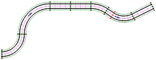
When the country 'United States of America' and the Design code 'AASHTO LRFD 7th Ed', is selected on the main Vehicle Load Optimisation dialog, road traffic loading data and parameters can be specified with reference to AASHTO LRFD Bridge Design Specifications, Seventh Edition.
 Loading
to AASHTO LRFD 7th Edition uses LUSAS Traffic Load Optimisation (TLO).
For this, the LUSAS model can be defined in any quadrant of the
Modeller view window. LUSAS TLO vehicle loads can be projected in
either X, Y or Z directions, meaning that models can now lie in any of
the primary (X,Y), (Y,Z) or (Z,X) planes. Consecutive straight lines
and arcs can also be used to define kerb positions. Loading
to AASHTO LRFD 7th Edition uses LUSAS Traffic Load Optimisation (TLO).
For this, the LUSAS model can be defined in any quadrant of the
Modeller view window. LUSAS TLO vehicle loads can be projected in
either X, Y or Z directions, meaning that models can now lie in any of
the primary (X,Y), (Y,Z) or (Z,X) planes. Consecutive straight lines
and arcs can also be used to define kerb positions.
Design codes are also available for many US State Bridge Design Manuals' implementations of AASHTO LRFD.
Canada CAN/CSA-S6-06
When the country 'Canada' and Design code 'CAN/CSA-S6-06 (Design)', is selected on the main Vehicle Load Optimisation dialog, road traffic loading is generated with reference to CAN/CSA-S6-06 Section 3. The scope of the vehicle load optimisation to CAN/CSA-S6-06 is restricted to vertical highway traffic loading and global effects. Horizontal components, railway loads and pedestrian loads are not currently included.
Onerous results tables
For design codes supported by LUSAS TLO only, and when a VLO analysis is run, a VLO onerous effects table can be optionally displayed which shows sorted results for all chosen influences at nodes that are visible, with the most onerous result shown in the first row of the table. A results tab is present for each
<Influence attribute - Sign - Design Case> group listed. This group is referred to as an 'Influence Design Loadcase'. Load patterns can be created on a case-by-case basis if not already created during the creation of the onerous effects table via a setting on the main VLO dialog.
Non-planar decks supported
LUSAS Traffic Load Optimisation now supports non-planar decks.
Results-related improvements
Construction tables
The construction table facility can be used to produce Camber, Displacement History, and Incremental Displacement tables of results for selected locations (points) on the model, and for any specified results loadcases. It is available for selected LUSAS Civil & Structural and LUSAS Bridge software products only. It is accessed from the Civil >or Bridge > Construction Table... menu item.
- Camber tables are used to set-out a structure towards a target (as-built) profile while accounting for effects during construction, such as dead-load deflection, creep and concrete shrinkage. Displacement values in a Camber table are absolute values with reference to an undeformed geometry 'datum'. They are effectively the reverse of Displacement History tables.
- Displacement History tables report the absolute displacement of a series of key-points at each stage with reference to an undeformed geometry 'datum'. This information could be used, for example, when constructing reinforced earthwork ramps, to determine the settlement at each rise and the required flexibility of transition slabs, or the total displacement of specified points throughout the construction of a bridge after each construction stage.
- Incremental Displacement History tables report on the stage-by-stage deformation of a structure. They tabulate the relative displacements between each construction stage, which can then be used in geometry control of structures built using sequential construction methods.

See Construction Table
reporting in action:
Feature based results
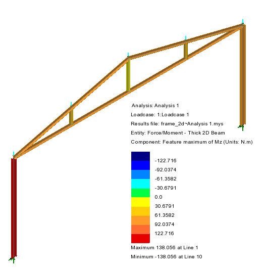
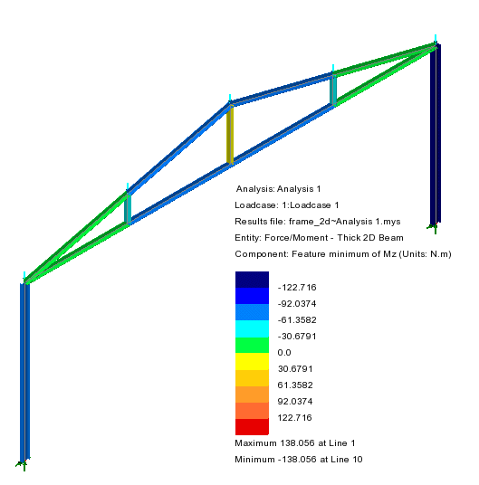
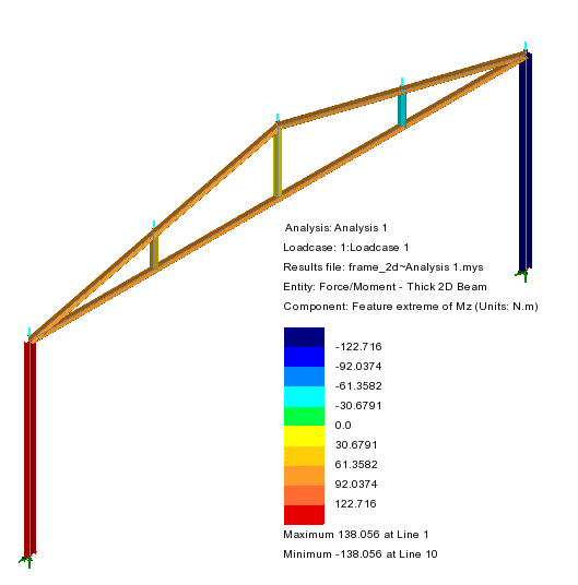
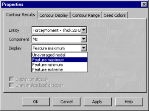 Results can now be displayed for contours on a feature basis, by making an appropriate selection on the relevant layer properties dialog: Results can now be displayed for contours on a feature basis, by making an appropriate selection on the relevant layer properties dialog:
- Feature maximum - for this, the whole of each feature (line, surface etc) is drawn in the same contour colour and in a colour that relates to the single highest value found in any node / element within that feature.
- Feature minimum -
for this, the whole of each feature (line, surface etc) is drawn in the same contour colour and in a colour that relates to the single lowest value found in any node / element within that feature, where the lowest value may be a positive or negative number.
- Feature extreme - contours the value with the largest magnitude and preserves its sign.
Feature maximum, minimum and extreme results can also be printed and output to reports.
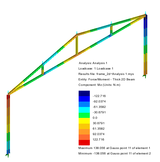
Example feature-based results contour plots are shown below.
|
|
|
|
Unaveraged nodal results
|
Contours of Feature maximum
|
|
|
|
|
Contours of Feature minimum
|
Contours of Feature extreme
|
|
Maximum / Minimum / Extreme results
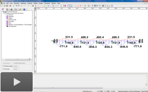
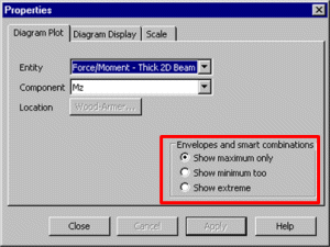 When viewing 'Max' results for an active envelope or a smart combination, Contours, Diagrams or Values plots can now show maximum, maximum and minimum, or 'extreme' results. Radio buttons on the relevant properties dialogs provide the options to: When viewing 'Max' results for an active envelope or a smart combination, Contours, Diagrams or Values plots can now show maximum, maximum and minimum, or 'extreme' results. Radio buttons on the relevant properties dialogs provide the options to:
- Show maximum only - ignores minimum values.
- Show minimum too - shows maximum and minimum values.
- Show extreme values This considers both the maximum and minimum value at each location, taking the larger absolute numerical value in each case, and preserving the sign of whichever value is used.
Note that when viewing 'Min' results for an active envelope or a smart combination the options provided will change to Show minimum only, and Show Maximum too.
For Diagram plots the maximum and minimum sections of the diagrams are drawn in different (user-definable) colours from the default orange colour used for standard diagram plots. By default red is used for maximum values, blue for minimum.
For Values plots maximum values are drawn in red, and minimum values are drawn in blue.
|
Examples:
|
For an Envelope (Min) loadcase:

|
|

|
|

|
See Maximum / Minimum / Extreme results
in action:
Graphing improvements
When the Graph Wizard has been successfully completed, the defined graph wizard utility name denoted by this icon  and its associated graph datasets and its associated graph datasets  are now added to the Utilities are now added to the Utilities  Treeview, and the chosen graph data is displayed. A context menu for the named graph wizard utility Treeview, and the chosen graph data is displayed. A context menu for the named graph wizard utility  includes the following menu items: includes the following menu items:
- Edit Attribute provides access to the settings made in defining the graph.
- Auto-update provides a switch to turn on / turn off automatic updating of the graph if the model or results have changed since a graph and its datasets were last displayed. Graphs set to not auto-update are shown by a locked graph icon
 . .
- Show graph allows predefined graphs to re-displayed at any time, without the wizard having to be re-accessed. Double-clicking on the named Graph wizard utility name denoted by this icon
 in the Utilities in the Utilities  Treeview, does the same. Treeview, does the same.
On the Graph view window, toolbar buttons provide the means to print, add a graph to a report  , edit the graph data , edit the graph data  , or edit its general properties and style , or edit its general properties and style  . .
Print Results Wizard
The Print Results Wizard now supports feature maximum, feature minimum and feature extreme results, and the printing of extreme envelope / smart combination results.
After making appropriate selections in the Print Results Wizard a Print Results Wizard  table entry is now added to the Utilities table entry is now added to the Utilities  Treeview to enable the results data to re-displayed at any time (if the view containing it was closed for any reason) without the wizard having to be re-accessed. Treeview to enable the results data to re-displayed at any time (if the view containing it was closed for any reason) without the wizard having to be re-accessed.
A context menu for Print Results Wizard  table entry in the Utilities table entry in the Utilities  Treeview entry includes the following menu items: Treeview entry includes the following menu items:
- Edit Attribute provides access to the settings made in defining the results data listing.
- Show Results allows predefined tables of results data to re-displayed at any time, without the wizard having to be re-accessed. Double-clicking on the named Print Results Wizard
 table entry in the Utilities table entry in the Utilities  Treeview does the same. Treeview does the same.
On the Printed Results table view window, toolbar buttons provide the means to save, print, or edit its general properties.
Threshold values
The ability to specify a threshold value has been added to relevant dialogs seen when using the
new Construction Table facility, the Print Results Wizard, or when generating reports.
A threshold value is an absolute value, up to which, all values between zero and the threshold value will be written or reported as zero.
One-click reports for selected features / objects
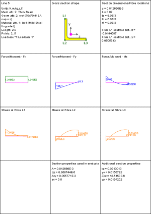
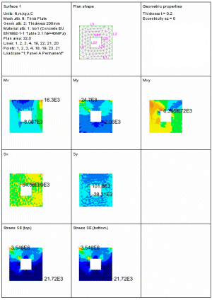
The new one-click report facility creates a one-page modelling and results summary for each selected feature showing a graphical representation of primary load effects on that feature or object for the active
loadcase. In its simplest form a one-click report is created by first selecting a line or surface (or element) in the model and then selecting the context menu item One-click report... for that feature. Multiple features (but only of the same type) can also be selected and be reported upon, and in this situation a multi-page summary would be created instead.
One-click reports can be printed off individually or be added to as individual chapters to
main reports. Each time a main report is generated the contents of a one-click report are updated to reflect the current state of the model and any corresponding results, if referenced by the report.
The one-click report facility can also be accessed from the Utilities > One-click report menu item, or from the One-click report  toolbar button. toolbar button.
Example pages:
|
|
|
|
One-click report for a line beam member (2D thick beam template)
|
One-click report for a surface (2D thick plate template)
|
Main Report enhancements
Maximum / Minimum / Extreme results
Feature maximum, feature minimum or feature extreme results for any loadcase, and extreme envelope /smart combination results can now be included in a report.
Graphs
Graphs defined by Graph Wizard Utility can be added to a report as a report chapter either at the time of their creation, or as part of adding a report chapter. Graphs that were defined and added to the Utilities  Treeview are initially listed in the Graphs panel of the report Chapters dialog. The name of a graph is automatically used as a title for the graph in the report. Treeview are initially listed in the Graphs panel of the report Chapters dialog. The name of a graph is automatically used as a title for the graph in the report.
Each time a report is generated the contents of a graph chapter are updated to reflect the current state of the model and/or results referenced by the graph, unless auto-update for the graph has been turned off.
Saved views
Saved views of the current view can be added to a report as a report chapter. Any saved views that were defined and added to the Utilities  Treeview are initially listed in the Saved view panel of the Chapters dialog. Check (tick) the appropriate views to include the contents of that view as a chapter in the report. Note that a title for the view is automatically added beneath the inserted image of the view in the report. This title is comprised of the view name followed by a loadcase name in parenthesis as, for example, 'Contours Fx (Loadcase 1)'. Treeview are initially listed in the Saved view panel of the Chapters dialog. Check (tick) the appropriate views to include the contents of that view as a chapter in the report. Note that a title for the view is automatically added beneath the inserted image of the view in the report. This title is comprised of the view name followed by a loadcase name in parenthesis as, for example, 'Contours Fx (Loadcase 1)'.
Each time a report is generated the contents of a saved view chapter are updated to reflect the current state of the model and/or results referenced by the saved view.
One-click reports
One-click reports can be added to as individual chapters to
main reports. With the on-screen one-click report displayed press the Add to report
 button. Pages to be inserted can be selected, along with the position within a report where they are to be added.
Each time a main report is generated the contents of a one-click report are updated to reflect the current state of the model and any corresponding results, if referenced by the report. button. Pages to be inserted can be selected, along with the position within a report where they are to be added.
Each time a main report is generated the contents of a one-click report are updated to reflect the current state of the model and any corresponding results, if referenced by the report.
Updated icons
The icons used in the Report  Treeview now comprise: Treeview now comprise:
 Main report entry
 Model or results chapter
 Image entry (chapter) - note that user-inserted image data does not update each time report is generated
 Saved view entry (chapter) - note that all saved views do update each time a report is generated
 One-click report entry (chapter)
 Graph entry (chapter) Graph entry (chapter)
Element-related improvements
2D/3D Bars
Geometric nonlinear co-rotational formulation has been added to 2D and 3D bar elements BAR2, BRS2 , BAR3 and BRS3 to improve the results obtained for these elements.
3D Thick Beams
Geometric nonlinear, Total Lagrangian and co-rotational formulation has been added to the BMI21, BMI31, BMX21 and BMX31 3D thick beam elements to improve the results obtained for these elements.
3D Thick shells
The performance of TTS3 and TTS6 thick shell elements has been improved. The introduction of assumed transverse shear strains significantly improves the TTS3 element, and also the TTS6 element. TTS3 is now insensitive to slenderness or mesh distortion, and shear oscillations are reduced. The stability of the 4-node QTS4 element for very thin shells discretised into coarse distorted meshes, has also been generally improved by using a correction to the formulation used.
Material model-related improvements
Piecewise Linear Hysteresis and Compound Hysteresis Joint Models
New Piecewise Linear Hysteresis and Compound Hysteresis Joint Models in this release are generic extensions of the Piecewise Linear Elastic Joint Model within LUSAS, and generalisations of well-known named hysteresis models that are in use in industry.
Applications include seismic analysis and soil joint modelling.
The primary backbone under monotonic loading is a piecewise linear curve as used by the Multi-linear Elastic Joint Model, where the whole loop for all multi-linear hysteresis joint models can be above or below the zero force axis, and the origin of the loop may have any displacement and force, not necessarily zero displacement and force.
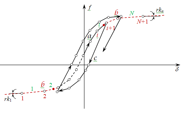
Piecewise linear curve with hysteresis behaviour.
Hysteretic models commonly used in industry can be defined by specifying a LUSAS hysteresis model type and a suitable unloading rule(s).
Industry models supported in this way include:
- Degrading bi-linear
- Bi-linear with slackness
- Origin-centred bi-linear
- Peak oriented
|
- Kivell degrading stiffness
- Pivotal plastic model
- Modified Takeda
- Muto degrading tri-linear
|
- Fukada degrading tri-linear
- Sina degrading trilinear
- Stewart degrading stiffness
- Franchin
|
It should be noted that, where industry-named models consist of a fixed number of piecewise linear segments to describe the primary
backbone of the curve, the implementation of the named hystereris models within LUSAS allows for multiple segments to be specified (if required) for each required line segment of a named model. In addition, various unloading rules can be chosen for a single hysteresis model, and any two basic hysteresis models may be combined with different loading and unloading rules to create compound hysteresis loops. This provides many options and permutations for assessing a wide variety of hysteretic joints.
|
|
|
|
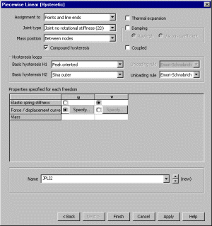
Piecewise linear hysteretic joint material dialog settings
for a Sina degrading trilinear model
|
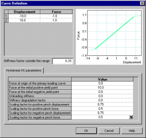
Defining force / displacement values and hysteresis parameters
|
|
|
|
|
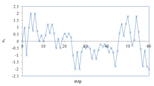
Applied displacement history
|
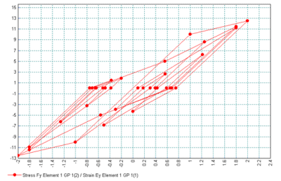
Variation of joint force with displacement
|
Modelling-related improvements
Saved views
A view of a model may now be saved by name into the Utilities  treeview using the Window > Save
View menu item. Views saved in this way are always retained and available when a model is saved, or when a model containing them is opened in a higher version of LUSAS. treeview using the Window > Save
View menu item. Views saved in this way are always retained and available when a model is saved, or when a model containing them is opened in a higher version of LUSAS.
Saved views have two primary uses:
- Saved View
 entries in the Utilities entries in the Utilities  treeview can be dragged and dropped onto any View window to automatically update the view settings and the display in that View window to those contained in the saved view. A Saved view entry can also be assigned to a New window or the Current window by using the respective Apply to> context menu items. Using these methods a number of standard model or results views can be set-up for easy and quick viewing of the predefined views of the model and of selected results plots. treeview can be dragged and dropped onto any View window to automatically update the view settings and the display in that View window to those contained in the saved view. A Saved view entry can also be assigned to a New window or the Current window by using the respective Apply to> context menu items. Using these methods a number of standard model or results views can be set-up for easy and quick viewing of the predefined views of the model and of selected results plots.
- Saved views can also be inserted into
reports, and when done, will ensure that the report, when generated, will always contain up-to-date images of any model or results plots because the image data contained in a saved view is re-generated each time a report is created. Note that the saved view name is automatically used as the title for the inserted image of the view in a generated report. This title is comprised of the view name followed by a loadcase name in parenthesis. For a default view name and loadcase name the inserted image of a saved view in a report would be titled: 'View1 (Loadcase 1)'. As a result it makes sense to name a saved view explicitly according to the contents of the view, for example, 'Isometric view' or 'Contours of Mz'.
Easier introduction of joints at the ends of
lines
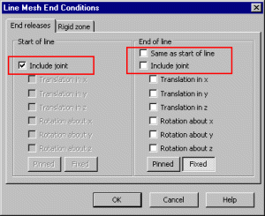 Joint elements can be automatically introduced at the ends of lines meshed with the grillage element or any of the 3D beam elements. This is done by selecting the �Include joint� check box on the Line Mesh End Conditions dialog for a line mesh attribute. The axes of the included joint are automatically aligned to the x,y and z beam axes of the beam to which they are assigned and the inserted joints are given default linear joint material properties based upon the material and geometric properties of the line on which they occur. Joint elements can be automatically introduced at the ends of lines meshed with the grillage element or any of the 3D beam elements. This is done by selecting the �Include joint� check box on the Line Mesh End Conditions dialog for a line mesh attribute. The axes of the included joint are automatically aligned to the x,y and z beam axes of the beam to which they are assigned and the inserted joints are given default linear joint material properties based upon the material and geometric properties of the line on which they occur.
If required, different joint material properties can be defined and assigned to relevant ends of lines to overwrite the default joint
values.
This new method greatly simplifies and speeds-up the insertion of joints for line features meshed with the stated element
types.
Rigid zones
When modelling the connection between beams and columns in a steel or concrete building frame, a short rigid length of beam element may be required to model the length of the beam that extends from the nodal intersection with one beam or column - the 'intersection of interest', to a position on the beam that defines the extent of a rigid zone for modelling and analysis purposes.
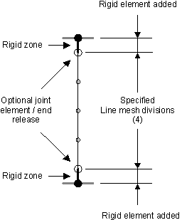
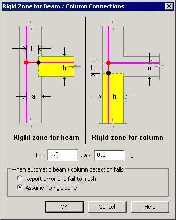
Rigid zones can be specified when defining a Line mesh attribute using the Attributes > Mesh > Line menu item. Different properties can be defined for the start and/or end of a line mesh attribute, and rigid zone lengths can be user-defined or
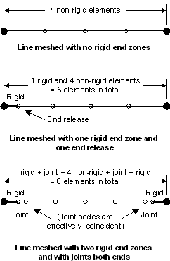
calculated according to a formula based upon the width and depth of intersecting beam and column members. Additional rigid elements (of the same type as the line element itself) are inserted at the start and / or end of each line mesh 'set' of spacings, but the inclusion of rigid end zones in a line mesh attribute does not change the number of line mesh divisions that were defined for that element. The defined number of line mesh divisions are fitted to the length of line that remains when any rigid end zones have been defined. Rigid zones receive the same loading as the non-rigid elements assigned to a line.
|
|
|
|
Line meshing options showing introduction of rigid zones
for columns and beams
|
Examples of line meshing with rigid zones
|
Formula based rigid zone calculation dialog
|
Visualisation of rigid zones
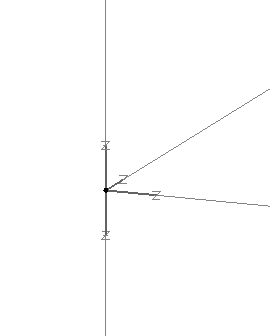
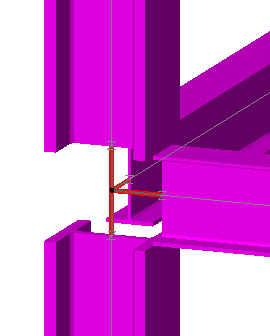
Rigid zone lengths are visualised on the Mesh layer as a thicker line and in a darker colour of the specified mesh colour. Defining rigid zones changes the fleshed length of beam sections. The following image shows what is displayed in each case.
|
|
|
|
Mesh layer visualisation of connection with rigid zones
(Rigid zone lengths are shown in thicker line style)
|
Fleshed geometry visualisation of connection with rigid zones
(Rigid zone lengths are drawn in same colour as the point colour)
|
Distributed perimeter loading
Distributed perimeter loading is a new load type that can be applied to unmeshed surfaces that represent a floor in a frame model. The loading applied is distributed to the edge beams based upon the spanning direction of the floor and any definition of sub-beams.
It is primarily of use in loading concrete floor slabs in buildings, where the floor panel itself is not modelled in full in order to reduce the complexity of the model. Surfaces representing the extent of each floor slab must be defined but no mesh assignment is required. Lines forming the Surface must, however, be assigned a suitable line mesh. Sub-beams that may support a floor slab (other than those beams that support its perimeter) can be defined without the need to model those beams as line features or elements in the model. Loading on sub-beams as a result of distributed slab loading and their self weight is represented as equivalent loads at the locations where the sub-beams meet the supporting beams at the perimeter of a surface.
|
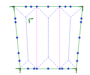
Two-way distributed loading with 2 sub-beams
|
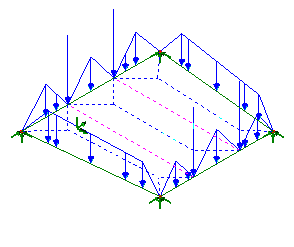
Perimeter loading generated
|
Real-time graphing of data
Real-time graphing of entered data (as already provided for the definition of tendon profiles) is also now provided when defining Load Curves, Response Spectra, and Piecewise linear joint material models.
General improvements
Import of third-party model data
Basic data from supported third-party
model data input files can be imported to create a feature-based geometry model using the File >
Import... menu item or a mesh-only model by using the File > Import Mesh menu item. When a file is selected the Advanced
button can be used to specify import parameters.
Note that the amount of usable modelling data provided in third party input files (meshing parameters, material and geometric property data and other attributes) varies according to each software package.
New feature/object selection cursors
New planar cursor selection options can be used to define planes in which, or axes along which, features can be selected. When used in isolation all features/objects in a chosen axis or plane will be selected within a cursor selection. When a planar cursor option is set prior to using a Feature/Mesh Object Selection option, individual points or lines or elements etc can be selected within the axis or plane chosen.
Axes and planes are defined by model view axes and the model
vertical axis.
| Specific cursor |
Notes |
 Select Vertical
 |
Select features/objects that are vertical with respect to the model vertical axis |
 Select Horizontal
 |
Select features/objects that are horizontal with respect to the model vertical axis |
 Select X axis
 |
Select features/objects in the X direction only and in relation to any active local coordinate set |
 Select Y axis
 |
Select features/objects in the Y direction only and in relation to any active local coordinate set |
 Select Z axis
 |
Select features/objects in the Z direction only and in relation to any active local coordinate set |
 Select XY plane
 |
Select features/objects that are in the XY plane and in relation to any active local coordinate set |
 Select YZ plane
 |
Select features/objects that are in the YZ plane and in relation to any active local coordinate set |
 Select XZ plane
 |
Select features/objects that are in the XZ plane and in relation to any active local coordinate set |
OpenGL speed-up
Various improvements to the OpenGL implementation result in:
- Improved selection / display speed / dynamic rotation of model data, where for various large test models with numerous loading arrows (e.g. gravity arrows) display speeds were 25x to 350x faster.
- Improved drawing of text in all situations and improved support for all character sets.
- New advanced software acceleration option provided as part of the
LUSAS Configuration Utility in addition to existing Hardware and Standard software options.
Other user change requests
In addition to the range of new facilities and improvements listed, many user change requests have also been implemented. The originators of all requested changes to the software (some of which are included in the above list of enhancements) have been incorporated in this release will be notified individually.
User Manuals
All online and printed documentation has been updated for this new release. Manuals are provided in PDF format as part of any V15 software download file or on the V15 software DVD.
Worked Examples
All worked examples have been updated for this release to ensure that the examples match changes made to the software and (when possible) to illustrate new facilities.
Manuals of Worked Examples are provided in PDF format as part of the LUSAS software download file or release DVD.
Potential issues opening PDF files referenced in CHM files
On some PCs, and for certain operating systems, the installation of security updates as released by Microsoft can affect the opening of PDF files from the table of contents panel within the CHM file-based help system. Any links to PDF files from within help topic pages may similarly be affected. If problems are found when attempting to open these files from within the online CHM file supplied please note the following:
- All manuals are supplied in PDF format on the installation kit and these are normally installed into the <LUSAS Installation Folder>/Programs/PDF_Manuals folder.
- Workarounds/solutions may be provided by Microsoft during the availability and support of this particular LUSAS software release.
- LUSAS is looking at producing online help in alternative formats.
Retired elements, material models and facilities
|